


This post is also available as a Python notebook.
From September 2017 to October 2018, I worked on TensorFlow 2.0 alongside many engineers. In this post, I’ll explain what TensorFlow 2.0 is and how it differs from TensorFlow 1.x. Towards the end, I’ll briefly compare TensorFlow 2.0 to PyTorch 1.0. This post represents my own views; it does not represent the views of Google, my former employer.
TensorFlow (TF) 2.0 is a significant, backwards-incompatible update to TF’s execution model and API.
Execution model. In TF 2.0, all operations execute imperatively by default. Graphs and the graph runtime are both abstracted away by a just-in-time tracer that translates Python functions executing TF operations into executable graph functions. This means in TF 2.0, there is no Session, and no global graph state. The tracer is exposed as a Python decorator, tf.function. This decorator is for advanced users. Using it is completely optional.
API. TF 2.0 makes tf.keras the high-level API for constructing and training neural networks. But you don’t have to use Keras if you don’t want to. You can instead use lower-level operations and automatic differentiation directly.
To follow along with the code examples in this post, install the TF 2.0 alpha.
pip install tensorflow==2.0.0-alpha0import tensorflow as tf
tf.__version__'2.0.0-alpha0'Contents
- Why TF 2.0?
- Imperative execution
- State
- Automatic differentiation
- Keras
- Graph functions
- Comparison to other Python libraries
- Domain-specific languages for machine learning
I. Why TF 2.0?
TF 2.0 largely exists to make TF easier to use, for newcomers and researchers alike.
TF 1.x requires metaprogramming
TF 1.x was designed to train extremely large, static neural networks. Representing a model as a dataflow graph and separating its specification from its execution simplifies training at scale, which explains why TF 1.x uses Python as a declarative metaprogramming tool for graphs.
But most people don’t need to train Google-scale models, and most people find metaprogramming difficult. Constructing a TF 1.x graph is like writing assembly code, and this abstraction is so low-level that it is hard to produce anything but the simplest differentiable programs using it. Programs that have data-dependent control flow are particularly hard to express as graphs.
Metaprogramming is (often) unnecessary
It is possible to implement automatic differentiation by tracing computations while they are executed, without static graphs; Chainer, PyTorch, and autograd do exactly that. These libraries are substantially easier to use than TF 1.x, since imperative programming is so much more natural than declarative programming. Moreover, when training models with large operations on a single machine, these graph-free libraries are competitive with TF 1.x performance. For these reasons, TF 2.0 privileges imperative execution.
Graphs are still sometimes useful, for distribution, serialization, code generation, deployment, and (sometimes) performance. That’s why TF 2.0 provides the just-in-time tracer tf.function, which transparently converts Python functions into functions backed by graphs. This tracer also rewrites tensor-dependent Python control flow to TF control flow, and it automatically adds control dependencies to order reads and writes to TF state. This means that constructing graphs via tf.function is much easier than constructing TF 1.x graphs manually.
Multi-stage programming
The ability to create polymorphic graph functions via tf.function at runtime makes TF 2.0 similar to a multi-stage programming language.
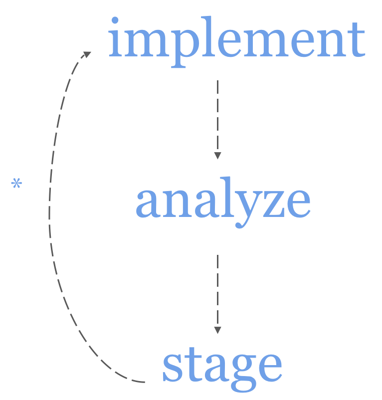
For TF 2.0, I recommend the following multi-stage workflow. Start by implementing your program in imperative mode. Once you’re satisfied that your program is correct, measure its performance. If the performance is unsatisfactory, analyze your program using cProfile or a comparable tool to find bottlenecks consisting of TF operations. Next, refactor the bottlenecks into Python functions, and stage these functions in graphs with tf.function.
If you mostly use TF 2.0 to train large deep models, you probably won’t need to analyze or stage your programs. If on the other hand you write programs that execute lots of small operations, like MCMC samplers or reinforcement learning algorithms, you’ll likely find this workflow useful. In such cases, the Python overhead incurred by executing operations eagerly actually matters.
II. Imperative execution
In TF 2.0, all operations are executed imperatively, or “eagerly”, by default. If you’ve used NumPy or PyTorch, TF 2.0 will feel familiar. For example, the following line of code will immediately construct two tensors backed by numerical tensors and then execute the add operation.
tf.constant([1., 2.]) + tf.constant([3., 4.])<tf.Tensor: id=1440, shape=(2,), dtype=int32, numpy=array([4, 6], dtype=float32)>Contrast the above code snippet to its verbose, awkward TF 1.x equivalent:
# TF 1.X code
x = tf.placeholder(tf.float32, shape=[2])
y = tf.placeholder(tf.float32, shape=[2])
value = x + y

with tf.Session() as sess:
  print(sess.run(value, feed_dict={x: [1., 2.], y: [3., 4.]}))
In TF 2.0, there are no placeholders, no sessions, and no feed dicts. Because operations are executed immediately, you can use (and differentiate through) if statements and for loops (no more tf.cond or tf.while_loop). You can also use whatever Python data structures you like, and debug your programs with print statements and pdb.
If TF detects that a GPU is available, it will automatically run operations on the GPU when possible. The target device can also be controlled explicitly.
if tf.test.is_gpu_available():
  with tf.device('gpu:0'):
    tf.constant([1., 2.]) + tf.constant([3., 4.])
III. State
Using tf.Variable objects in TensorFlow required wrangling global collections of graph state, with confusing APIs like tf.get_variable, tf.variable_scope, and tf.initializers.global_variables. TF 2.0 does away with global collections and their associated APIs. If you need a tf.Variable in TF 2.0, then you just construct and initialize it directly:
tf.Variable(tf.random.normal([3, 5]))<tf.Variable 'Variable:0' shape=(3, 5) dtype=float32, numpy=
array([[ 0.13141578, -0.18558209, 1.2412338 , -0.5886968 , -0.9191646 ],
[ 1.186105 , -0.45135704, 0.57979995, 0.12573312, -0.7697861 ],
[ 0.28296474, 1.2735683 , -0.08385598, 0.59388596, -0.2402552 ]],
dtype=float32)>IV. Automatic differentiation
TF 2.0 implements reverse-mode automatic differentiation (also known as backpropagation), using a trace-based mechanism. This trace, or tape, is exposed as a context manager, tf.GradientTape. The watch method designates a Tensor as something that we’ll need to differentiate with respect to later. Notice that by tracing the computation of dy_dx under the first tape, we’re able to compute d2y_dx2.
x = tf.constant(3.0)
with tf.GradientTape() as t1:
  with tf.GradientTape() as t2:
    t1.watch(x)
    t2.watch(x)
    y = x * x
  dy_dx = t2.gradient(y, x)
d2y_dx2 = t1.gradient(dy_dx, x)dy_dx<tf.Tensor: id=62, shape=(), dtype=float32, numpy=6.0>d2y_dx2<tf.Tensor: id=68, shape=(), dtype=float32, numpy=2.0>tf.Variable objects are watched automatically by tapes.
x = tf.Variable(3.0)
with tf.GradientTape() as t1:
  with tf.GradientTape() as t2:
    y = x * x
  dy_dx = t2.gradient(y, x)
d2y_dx2 = t1.gradient(dy_dx, x)
V. Keras
TF 1.x is notorious for having many mutually incompatible high-level APIs for neural networks. TF 2.0 has just one high-level API: tf.keras, which essentially implements the Keras API but is customized for TF. Several standard layers for neural networks are available in the tf.keras.layers namespace.
Keras layers can be composed via tf.keras.Sequential() to obtain an object representing their composition. For example, the below code trains a toy CNN on MNIST. (Of course, MNIST can be solved by much simpler methods, like least squares.)
mnist = tf.keras.datasets.mnist
(x_train, y_train), (x_test, y_test) = mnist.load_data()
input_shape=[28, 28, 1]
data_format="channels_last"

max_pool = tf.keras.layers.MaxPooling2D(
      (2, 2), (2, 2), padding='same', data_format=data_format)

model = tf.keras.Sequential([
  tf.keras.layers.Reshape(target_shape=input_shape,
    input_shape=[28, 28]),
  tf.keras.layers.Conv2D(32,5,
    padding='same', data_format=data_format,
    activation=tf.nn.relu),
  max_pool,
  tf.keras.layers.Conv2D(64, 5,
    padding='same', data_format=data_format,
    activation=tf.nn.relu),
  max_pool,
  tf.keras.layers.Flatten(),
  tf.keras.layers.Dense(1024, activation=tf.nn.relu),
  tf.keras.layers.Dropout(0.3),
  tf.keras.layers.Dense(10, activation=tf.nn.softmax)
])
model.compile(optimizer=tf.optimizers.Adam(),
loss=tf.losses.sparse_categorical_crossentropy,
metrics=['accuracy'])model.fit(x_train, y_train, epochs=1)60000/60000 [==============================] - 238s 4ms/sample - loss: 0.3417 - accuracy: 0.9495Alternatively, the same model could have been written as a subclass of tf.keras.Model.
class ConvNet(tf.keras.Model):
  def __init__(self, input_shape, data_format):
    super(ConvNet, self).__init__()
    self.reshape = tf.keras.layers.Reshape(
      target_shape=input_shape, input_shape=[28, 28])
    self.conv1 = tf.keras.layers.Conv2D(32,5,
      padding='same', data_format=data_format,
      activation=tf.nn.relu)
    self.pool = tf.keras.layers.MaxPooling2D(
      (2, 2), (2, 2), padding='same', data_format=data_format)
    self.conv2 = tf.keras.layers.Conv2D(64, 5,
      padding='same', data_format=data_format,
      activation=tf.nn.relu)
    self.flt = tf.keras.layers.Flatten()
    self.d1 = tf.keras.layers.Dense(1024, activation=tf.nn.relu)
    self.dropout = tf.keras.layers.Dropout(0.3)
    self.d2 = tf.keras.layers.Dense(10, activation=tf.nn.softmax)

  def call(self, x):
    x = self.reshape(x)
    x = self.conv1(x)
    x = self.pool(x)
    x = self.conv2(x)
    x = self.pool(x)
    x = self.flt(x)
    x = self.d1(x)
    x = self.dropout(x)
    return self.d2(x)
If you don’t want to use tf.keras, you can use low-level APIs like tf.reshape, tf.nn.conv2d, tf.nn.max_pool, tf.nn.dropout, and tf.matmul directly.
VI. Graph functions
For advanced users who need graphs, TF 2.0 provides tf.function, a just-in-time tracer that converts Python functions that execute TensorFlow operations into graph functions. A graph function is a TF graph with named inputs and outputs. Graph functions are executed by a C++ runtime that automatically partitions graphs across devices, and it parallelizes and optimizes them before execution.
Calling a graph function is syntactically equivalent to calling a Python function. Here’s a very simple example.
@tf.function
def add(tensor):
  return tensor + tensor + tensor
# Executes as a dataflow graph
add(tf.ones([2, 2])) <tf.Tensor: id=1487, shape=(2, 2), dtype=float32, numpy=
array([[3., 3.],
[3., 3.]], dtype=float32)>The add function is also polymorphic in the data types and shapes of its Tensor arguments (and the run-time values of the non-Tensor arguments), even though TF graphs are not.
add(tf.ones([2, 2], dtype=tf.uint8)) <tf.Tensor: id=1499, shape=(2, 2), dtype=uint8, numpy=
array([[3, 3],
[3, 3]], dtype=uint8)>Every time a graph function is called, its “input signature” is analyzed. If the input signature doesn’t match an input signature it has seen before, it re-traces the Python function and constructs another concrete graph function. (In programming languages terms, this is like multiple dispatch or lightweight modular staging.) This means that for one Python function, many concrete graph functions might be constructed. This also means that every call that triggers a trace will be slow, but subsequent calls with the same input signature will be much faster.
Lexical closure, state, and control dependencies
Graph functions support lexically closing over tf.Tensor and tf.Variable objects. You can mutate tf.Variable objects inside a graph function, and tf.function will automatically add the control dependencies needed to ensure that your reads and writes happen in program-order.
a = tf.Variable(1.0)
b = tf.Variable(1.0)

@tf.function
def f(x, y):
  a.assign(y * b)
  b.assign_add(x * a)
  return a + b

f(tf.constant(1.0), tf.constant(2.0))
<tf.Tensor: id=1569, shape=(), dtype=float32, numpy=5.0>a<tf.Variable 'Variable:0' shape=() dtype=float32, numpy=2.0>b<tf.Variable 'Variable:0' shape=() dtype=float32, numpy=3.0>Python control flow
tf.function automatically rewrites Python control flow that depends on tf.Tensor data into graph control flow, using autograph. This means that you no longer need to use constructs like tf.cond and tf.while_loop. For example, if we were to translate the following function into a graph function via tf.function, autograph would convert the for loop into a tf.while_loop, because it depends on tf.range(100), which is a tf.Tensor.
def matmul_many(tensor):
  accum = tensor
  for _ in tf.range(100):  # will be converted by autograph
    accum = tf.matmul(accum, tensor)
  return accum
It’s important to note that if tf.range(100) were replaced with range(100), then the loop would be unrolled, meaning that a graph with 100 matmul operations would be generated.
You can inspect the code that autograph generates on your behalf.
print(tf.autograph.to_code(matmul_many))from __future__ import print_function
def tf__matmul_many(tensor):
try:
with ag__.function_scope('matmul_many'):
do_return = False
retval_ = None
accum = tensor
def loop_body(loop_vars, accum_1):
with ag__.function_scope('loop_body'):
_ = loop_vars
accum_1 = ag__.converted_call('matmul', tf, ag__.ConversionOptions(recursive=True, verbose=0, strip_decorators=(ag__.convert, ag__.do_not_convert, ag__.converted_call), force_conversion=False, optional_features=ag__.Feature.ALL, internal_convert_user_code=True), (accum_1, tensor), {})
return accum_1,
accum, = ag__.for_stmt(ag__.converted_call('range', tf, ag__.ConversionOptions(recursive=True, verbose=0, strip_decorators=(ag__.convert, ag__.do_not_convert, ag__.converted_call), force_conversion=False, optional_features=ag__.Feature.ALL, internal_convert_user_code=True), (100,), {}), None, loop_body, (accum,))
do_return = True
retval_ = accum
return retval_
except:
ag__.rewrite_graph_construction_error(ag_source_map__)
tf__matmul_many.autograph_info__ = {}Performance
Graph functions can provide significant speed-ups for programs that execute many small TF operations. For these programs, the Python overhead incurred executing an operation imperatively outstrips the time spent running the operations. As an example, let’s benchmark the matmul_many function imperatively and as a graph function.
graph_fn = tf.function(matmul_many)Here’s the imperative (Python) performance.
%%timeit

matmul_many(tf.ones([2, 2]))
100 loops, best of 3: 13.5 ms per loopThe first call to graph_fn is slow, since this is when the graph function is generated.
%%time

graph_fn(tf.ones([2, 2]))
CPU times: user 158 ms, sys: 2.02 ms, total: 160 ms
Wall time: 159 ms
<tf.Tensor: id=1530126, shape=(2, 2), dtype=float32, numpy=
array([[1., 1.],
[1., 1.]], dtype=float32)>But subsequent calls are an order of magnitude faster than imperatively executing matmul_many.
%%timeit

graph_fn(tf.ones([2, 2]))
1000 loops, best of 3: 1.97 ms per loopVII. Comparison to other Python libraries
There are many libraries for machine learning. Out of all of them, PyTorch 1.0 is the one that’s most similar to TF 2.0. Both TF 2.0 and PyTorch 1.0 execute imperatively by default, and both provide ways to transform Python functions into graph-backed functions (compare tf.function and torch.jit). The PyTorch JIT tracer, torch.jit.trace, doesn’t implement the multiple-dispatch semantics that tf.function does, and it also doesn’t rewrite the AST. On the other hand, TorchScript lets you use Python control flow, but unlike tf.function, it doesn’t let you mix in arbitrary Python code that parametrizes the construction of your graph. That means that in comparison to tf.function, TorchScript makes it harder for you to shoot yourself in the foot, while potentially limiting your creative expression.
So should you use TF 2.0, or PyTorch 1.0? It depends. Because TF 2.0 is in alpha, it still has some kinks, and its imperative performance still needs work. But you can probably count on TF 2.0 becoming stable sometime this year. If you’re in industry, TensorFlow has TFX for production pipelines, TFLite for deploying to mobile, and TensorFlow.js for the web. PyTorch recently made a commitment to production; since then, they’ve added C++ inference and deployment solutions for several cloud providers. For research, I’ve found that TF 2.0 and PyTorch 1.0 are sufficiently similar that I’m comfortable using either one, and my choice of framework depends on my collaborators.
The multi-stage approach of TF 2.0 is similar to what’s done in JAX. JAX is great if you want a functional programming model that looks exactly like NumPy, but with automatic differentiation and GPU support; this is, in fact, what many researchers want. If you don’t like functional programming, JAX won’t be a good fit.
VIII. Domain-specific languages for machine learning
TF 2.0 and PyTorch 1.0 are very unusual libraries. It has been observed that these libraries resemble domain-specific languages (DSLs) for automatic-differentiation and machine learning, embedded in Python (see also our paper on TF Eager, TF 2.0’s precursor). What TF 2.0 and PyTorch 1.0 accomplish in Python is impressive, but they’re pushing the language to its limits.
There is now significant work underway to embed ML DSLs in languages that are more amenable to compilation than Python, like Swift (DLVM, Swift for TensorFlow, MLIR), and Julia (Flux, Zygote). So while TF 2.0 and PyTorch 1.0 are great libraries, do stay tuned: over the next year (or two, or three?), the ecosystem of programming languages for machine learning will continue to evolve rapidly.
I great resumen, clear and very useful. Thanks!
Thank you very much for the post, very helpful.
Is there a way to use the tensoflow debugger with Keras?
You’re welcome! In TF 1.x, the TensorFlow Debugger can be used to inspect Keras models (see https://www.tensorflow.org/guide/debugger). But I’m not sure whether the TF debugger is supported in 2.0. Because everything executes eagerly in 2.0, you shouldn’t really need to use a TF-specific debugger — you can just use Python’s `pdb`.